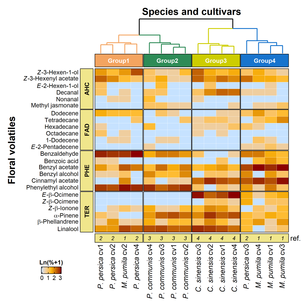
Heatmap is among the most popular ways of visualization for multivariant data analysis people use in their presentation and researches. In studies of metabolomics related to plants or insects, heatmap can be straightforward in comparing metabolites among treatments in both quantitative and qualitative manners. Here one example is shown about how to illustrate the chemical production of floral volatiles from four plant species, eaching having diffierent cultivars, using the Heatmap function in the ‘ComplexHeatmap’ packages in R. In this example the heatmap layout contains top, bottom and left annotation. The top annotation is hierarchical cluster analysis representing the dissimilarity/similarity of floral volatiles profiles (shift-log transformed prior to analysis) among the cultivars. The left annotation indicates the chemical classification (TER: terpenes; PHE: phenylpropanoids; FAD: fatty acid derivatives; HYD: aliphatic hydrocarbons) for the listed floral compounds. The bottom annotation is totally-customed, and in this case it provides numbers indicating cited literatures.
Load packages
library(ComplexHeatmap)
library(dendextend)
Load data:
table = ("
Volatiles Class MP001 MP002 MP003 MP004 PP001 PP002 PP003 PP004 PC001 PC002 PC003 PC004 CS001 CS002 CS003 CS004
E-b-Ocimene TER 3 0 4 1 0 0 4 0 0 0 0 0 12 9 18 25
Z-b-Ocimene TER 2 0 2 0 0 0 4 0 0 0 0 0 2 2 0 1
Z-b-Ionone TER 1 2 3 2 0 1 0 1 1 3 1 4 5 6 3 2
a-Pinene TER 4 0 3 2 2 1 3 0 11 8 9 5 9 14 6 11
b-Phellandrene TER 1 1 5 5 1 5 3 1 3 3 1 4 3 6 2 1
Linalool TER 1 12 2 0 5 5 3 9 9 9 12 11 11 13 15 8
Benzaldehyde PHE 4 14 3 7 16 14 7 23 7 5 7 4 0 0 2 1
'Benzoic acid' PHE 5 0 3 3 1 1 0 0 0 0 0 0 2 0 0 0
'Benzyl acetate' PHE 15 10 19 26 5 2 12 7 4 7 8 3 5 4 3 3
'Benzyl alcohol' PHE 5 2 2 0 1 1 6 0 3 6 3 6 2 2 0 1
'Cinnamyl acetate' PHE 11 6 18 15 0 0 10 0 1 1 0 2 11 15 8 9
'Phenylethyl alcohol' PHE 7 18 2 1 13 11 5 15 12 15 9 15 2 0 2 1
Z-3-Hexen-1-ol FAD 2 5 1 4 5 3 2 11 1 3 1 2 3 4 9 4
'Z-3-Hexenyl acetate' FAD 4 3 3 4 9 6 8 2 1 1 4 2 8 5 9 6
E-2-Hexen-1-ol FAD 1 0 0 0 2 0 0 0 0 0 3 0 0 2 0 0
Decanal FAD 1 1 0 1 2 0 1 0 0 0 2 2 9 6 2 8
Nonanal FAD 0 1 0 0 0 1 0 0 0 0 0 3 0 0 1 0
'Methyl jasmonate' FAD 1 0 2 1 0 0 0 0 1 1 2 2 0 0 0 1
Dodecene HYD 2 3 3 5 4 3 2 3 1 0 2 0 1 0 0 1
Tetradecane HYD 3 0 6 2 0 0 0 2 0 2 0 0 2 2 1 1
Hexadecane HYD 0 0 0 1 1 0 2 0 0 0 0 3 1 1 1 2
Octadecane HYD 0 1 0 0 2 0 0 0 0 0 0 0 1 0 1 0
1-Dodecene HYD 1 1 0 2 0 1 0 0 1 0 1 0 0 0 0 0
E-2-Pentadecene HYD 2 0 1 1 0 0 1 0 0 0 0 1 0 0 0 0
")
data <- read.table(textConnection(table),header=TRUE)
data.2 <- data[,c(-2)]
rownames(data.2) <- data.2[,1]
data.2[,1] <- NULL
data.2[,1]
col_lbs <- expression(
                      italic('M. pumila')~cv1,
                      italic('M. pumila')~cv2,
                      italic('M. pumila')~cv3,
                      italic('M. pumila')~cv4,
                      italic('P. persica')~cv1,
                      italic('P. persica')~cv2,
                      italic('P. persica')~cv3,
                      italic('P. persica')~cv4,
                      italic('P. communis')~cv1,
                      italic('P. communis')~cv2,
                      italic('P. communis')~cv3,
                      italic('P. communis')~cv4,
                      italic('C. sinensis')~cv1,
                      italic('C. sinensis')~cv2,
                      italic('C. sinensis')~cv3,
                      italic('C. sinensis')~cv4
                                               )
row_lbs <- expression(
italic('E')-beta-Ocimene,
italic('Z')-beta-Ocimene,
italic('Z')-beta-Ionone,
alpha*-Pinene,
beta-Phellandrene,
                      Linalool,
                      Benzaldehyde,
                      Benzoic~acid,
                      Benzyl~acetate,
                      Benzyl~alcohol,
                      Cinnamyl~acetate,
                      Phenylethyl~alcohol,
                      italic('Z')-3-Hexen-1-ol,
                      italic('Z')-3-Hexenyl~acetate,
                      italic('E')-2-Hexen-1-ol,
                      Decanal,
                      Nonanal,
                      Methyl~jasmonate,
                      Dodecene,
                      Tetradecane,
Hexadecane,
Octadecane,
1-Dodecene,
italic('E')-2-Pentadecene
                                               )
Plot heatmap
tiff("hmp.tiff", width = 7, height = 7, units = 'in', res = 300)
## global setting on some parametersht_opt(heatmap_column_title_gp = gpar(fontsize = 10),
legend_border = "black",
heatmap_border = TRUE,
annotation_border = TRUE )
## shift log transforamtion the matrix data.hmp <- data.matrix( log(data.2[,1:ncol(data.2)] + 1) )
## custom color of dend and of legendcol_dend = hclust( dist(t(data.hmp), method = "euclidean"),
method = "ward.D2" )
col_fun = circlize::colorRamp2( c(0, 1.5, 3),
c("slategray1", "darkgoldenrod1", "darkred") )
## custom bottom annotation ref = rep(c('1','2','3','4'), each = 4)
col_ref = c(rep("khaki",16)) ## use vectors with color names if preferring multiple colors
names(col_ref) = ref
Heatmap(
        data.hmp,
rect_gp = gpar(col = "white", lwd=0.1),
column_labels = col_lbs, # defined earlierrow_labels = row_lbs, # defined earlier
cluster_rows = FALSE,
row_split = c( rep("TER", 6), rep("PHE", 6), rep("FAD", 6),
rep("HYD", 6) ),
cluster_columns = color_branches(col_dend,
k=4, col = c('sandybrown','seagreen','yellow3','dodgerblue3') ), column_split = 4,
column_dend_height = unit(2, "cm"),
column_dend_gp = gpar(lwd = 2),row_gap = unit(0.4, "mm"),
column_gap = unit(0.4, "mm"),
top_annotation = HeatmapAnnotation(foo = anno_block(gp = gpar(fill = c('sandybrown','seagreen','yellow3','dodgerblue3'), lwd=1),
labels = c("Group1", "Group2", "Group3", "Group4"),
labels_gp = gpar(col = "white",
fontsize = 10,
fontface = "bold") ) ),
bottom_annotation = HeatmapAnnotation(ref. = anno_simple(ref,
col = col_ref,
pch = ref,
border = T,
pt_gp = gpar(col = "black",
fontsize = 9, fontface = 3) ) ), left_annotation = rowAnnotation(foo = anno_block(gp = gpar(fill = "khaki"),
labels = c("AHC","FAD", "PHE", "TER"),
labels_gp = gpar(col = "black",
fontsize = 10,
fontface = "bold") ) ),
row_title = "Floral volatiles",
column_title = "Species and cultivars",
row_title_gp = gpar(fontsize = 16, fontface = "bold"),
column_title_gp = gpar(fontsize = 16, fontface = "bold"),
row_names_side = "left",
column_names_gp = gpar(fontsize = 12, fontface = 'italic' ),
row_names_gp = gpar(fontsize = 10),
col = col_fun, # heatmap color scales defined earlier
heatmap_legend_param = list( title = "Ln(%+1)",border = "black",
direction = "horizontal",
title_position = "topcenter" ),
show_heatmap_legend = FALSE # remove the legend, since I would custom a legend and put it at specific location, see below
)
lgd = Legend(col_fun = col_fun, # same parameters with 'col' and 'heatmap_legend_param' both defined earlier
title = "Ln(%+1)",
border = "black",
direction = "horizontal",
title_position = "topcenter")
draw(lgd, x = unit(3, "cm"), y = unit(2, "cm"), ) ## display legend at specific positiondev.off()